import os

import numpy as np
import pandas as pd
import plotnine as p9
import matplotlib.colors
import scipy.stats as stats
import matplotlib.pyplot as plt

from IPython.display import Image
from mizani.formatters import percent_formatIntegrating air microbiome for comprehensive air quality analysis
An evaluation of the potential of HVS for airborne microbiome monitoring
Here, we conduct part of the analysis and generate figures for the manuscript Integrating the air microbiome for comprehensive air quality analysis.
To enhance readability, most of the code is hidden by default. You can expand it by clicking the “Show code” button above each cell. The complete code should be executable in a local environment, running smoothly from start to finish.
Preamble
Show code imports and presets
In this section we load the necessary libraries and set the global parameters for the notebook. It’s irrelevant for the narrative of the analysis but essential for the reproducibility of the results.
Imports
Pre-sets
# Matplotlib settings
import matplotlib.pyplot as plt
from matplotlib_inline.backend_inline import set_matplotlib_formats
plt.rcParams['font.family'] = 'Georgia'
plt.rcParams['svg.fonttype'] = 'none'
set_matplotlib_formats('retina')
plt.rcParams['figure.dpi'] = 300

# Plotnine settings (for figures)

p9.options.set_option('base_family', 'Georgia')

p9.theme_set(
    p9.theme_bw()
    + p9.theme(panel_grid=p9.element_blank(),
               legend_background=p9.element_blank(),
               panel_grid_major=p9.element_line(size=.5, linetype='dashed',
                                                alpha=.15, color='black'),
               plot_title=p9.element_text(ha='center'),
               dpi=300
    )
)

separator_line =  p9.annotate(
    geom='line',
    linetype='dashed',
    size=.2,
    x=[137, 144],
    y= [31, 36],
  )
Data loading and wrangling
We start by loading the medatata file which we have stored in /data/meta.txt with information about each sample:
metadata_df = pd.read_table('../data/meta.txt', sep='\t')
metadata_df.head()| Sample Name | Sample Number | AirLab_Code | Seq ID | Sample ID | Sampling | Project Name | Location | Relative Location | Media Type | ... | Entered By | DNA Extraction Date (YYYY-MM-DD) | DNA Extraction Kit | DNA Concentration (ng/uL) | DNA Volume of Elution (uL) | DNA Quantification Instrument | DNA Vol. Used for Quantification (uL) | DNA Storage Freezer | DNA Storage Drawer | DNA Performed By | |
|---|---|---|---|---|---|---|---|---|---|---|---|---|---|---|---|---|---|---|---|---|---|
| 0 | 2022/11/23HVS-SASS-PilotA1 | 1 | T6.0 B | HVSP1 | C6-B | Continuous | HVS-SASS-Pilot | AirLab Terrace | Outdoor | Quartz Filter | ... | Cassie Heinle | 28/11/2022 | Phe-Chlo method (AirLab Spain) | 7133 | 17 | Quantus Promega (AirLab Spain) | 5 | -20C MPL Freezer (New) | Yee Hui | AirLab Spain |
| 1 | 2022/11/28HVS-SASS-PilotA2 | 2 | T6.1 B | HVSP2 | D6.1-B | Discrete | HVS-SASS-Pilot | AirLab Terrace | Outdoor | Quartz Filter | ... | Cassie Heinle | 28/11/2022 | Phe-Chlo method (AirLab Spain) | 856 | 17 | Quantus Promega (AirLab Spain) | 5 | -20C MPL Freezer (New) | Yee Hui | AirLab Spain |
| 2 | 2022/11/28HVS-SASS-PilotA3 | 3 | T6.2 B | HVSP3 | D6.2-B | Discrete | HVS-SASS-Pilot | AirLab Terrace | Outdoor | Quartz Filter | ... | Cassie Heinle | 28/11/2022 | Phe-Chlo method (AirLab Spain) | 1193 | 17 | Quantus Promega (AirLab Spain) | 5 | -20C MPL Freezer (New) | Yee Hui | AirLab Spain |
| 3 | 2022/11/28HVS-SASS-PilotA4 | 4 | T6.3 B | HVSP4 | D6.3-B | Discrete | HVS-SASS-Pilot | AirLab Terrace | Outdoor | Quartz Filter | ... | Cassie Heinle | 28/11/2022 | Phe-Chlo method (AirLab Spain) | 1483 | 17 | Quantus Promega (AirLab Spain) | 5 | -20C MPL Freezer (New) | Yee Hui | AirLab Spain |
| 4 | 2022/11/28HVS-SASS-PilotA5 | 5 | T6.4 B | HVSP5 | D6.4-B | Discrete | HVS-SASS-Pilot | AirLab Terrace | Outdoor | Quartz Filter | ... | Cassie Heinle | 28/11/2022 | Phe-Chlo method (AirLab Spain) | 111 | 17 | Quantus Promega (AirLab Spain) | 5 | -20C MPL Freezer (New) | Yee Hui | AirLab Spain |
5 rows × 28 columns
metadata_df = (metadata_df
 .drop(columns=metadata_df.nunique().loc[lambda x: x==1].index)
 .rename(columns={'Seq ID': 'sample_id'})

)
The total read count for each assigned species across all samples is loaded from /data/REL_hvsp_sp.txt
species_df = pd.read_table('../data/REL_hvsp_sp.txt')Species identified as contaminants will be excluded from the analysis:
contamination_list = [
    "Galendromus occidentalis",
    "Bemisia tabaci",
    "Candidatus Portiera aleyrodidarum",
    "Frankliniella occidentalis",
    "Thrips palmi"
]
Information on the total DNA yield of each sample is stored in the /data/DNA.xlsx file:
dna_yields = (pd.read_excel('../data/DNA.xlsx')
 .rename(columns={
    'DNA Concentration (ng/uL)': 'dna_conc',
    'DNA Volume of Elution (uL)': 'dna_vol',
    'Sample ID': 'sample_code'
 })
 .assign(dna_yield=lambda x: x['dna_conc'] * x['dna_vol'])
 [['sample_code', 'dna_yield']]
)
We generate a long-form dataframe with the species counts for each sample:
species_long = (species_df
 .rename(columns={'#Datasets': 'name'})
 .melt('name', var_name='sample_id', value_name='reads')
 .assign(sample_id=lambda x: x['sample_id'].str.split('.').str[0])
 .query('name not in @contamination_list')
 .query('reads > 0')
)
species_long.sample(10)| name | sample_id | reads | |
|---|---|---|---|
| 100599 | Nocardioides islandensis | HVSP12 | 88.0 |
| 87172 | Granulibacter bethesdensis | HVSP11 | 38.0 |
| 152170 | Kaistella daneshvariae | HVSP19 | 68.0 |
| 164000 | Archangium violaceum | HVSP20 | 56.0 |
| 32121 | Pseudomonas cremoris | HVSP4 | 38.0 |
| 308929 | Haloechinothrix halophila | HVSP41 | 25.0 |
| 582584 | Arthrobacter sp. SX1312 | HVSP72 | 31.0 |
| 153999 | Sphingomonas sp. TZW2008 | HVSP19 | 42.0 |
| 236305 | Medicago truncatula | HVSP30 | 179.0 |
| 125319 | Novosphingobium sp. AP12 | HVSP15 | 64.0 |
Experiment 1: Continuous vs Discrete sampling
Let’s begin by examining how the DNA yield of each sample compares to the species diversity (measured as species richness):
Show Code
exp_1_samples = ['C3-B', 'D3.1-B', 'D3.2-B', 'D3.3-B', 'C6-B', 'D6.1-B', 'D6.2-B',
                  'D6.3-B', 'D6.4-B', 'D6.5-B', 'D6.6-B',]
exp1_names = [s.split('-')[0] for s in exp_1_samples]
exp_1_meta = (metadata_df
 .query('`Sample ID` in @exp_1_samples')
 .assign(sampling_days=lambda x: x['Sample ID'].str[1])
 .rename(columns={'Sample ID': 'sample_code', 'Sampling': 'mode'})
 [['sample_id', 'sample_code', 'mode', 'sampling_days']]
 .merge(dna_yields, on='sample_code')
)

(species_long
 .query('reads > 0')
 .groupby('sample_id')
 .size()
 .reset_index(name='richness')
 .merge(exp_1_meta)
 .assign(sample_code=lambda dd: dd.sample_code.str.split('-').str[0])
 .assign(sample_code=lambda dd:
         pd.Categorical(dd.sample_code, categories=exp1_names, ordered=True))
 .melt(id_vars=['sample_id', 'sample_code', 'mode', 'sampling_days'])
 .replace({'richness': 'Species richness', 'dna_yield': 'DNA yield (ng)'})
 .pipe(lambda x: p9.ggplot(x)
       + p9.aes(x='sample_code', y='value', fill='mode')
       + p9.geom_col()
       + p9.facet_wrap('~variable', scales='free_y', ncol=1)
       + p9.annotate('vline', xintercept=[4.5], linetype='dashed', size=.4)
       + p9.labs(x='', y='', fill='')
       + p9.theme(
           figure_size=(4, 4),
           axis_text_x=p9.element_text(angle=45),
           legend_position='top',
           legend_key_size=10,
           legend_text=p9.element_text(size=7),
           )
       )
)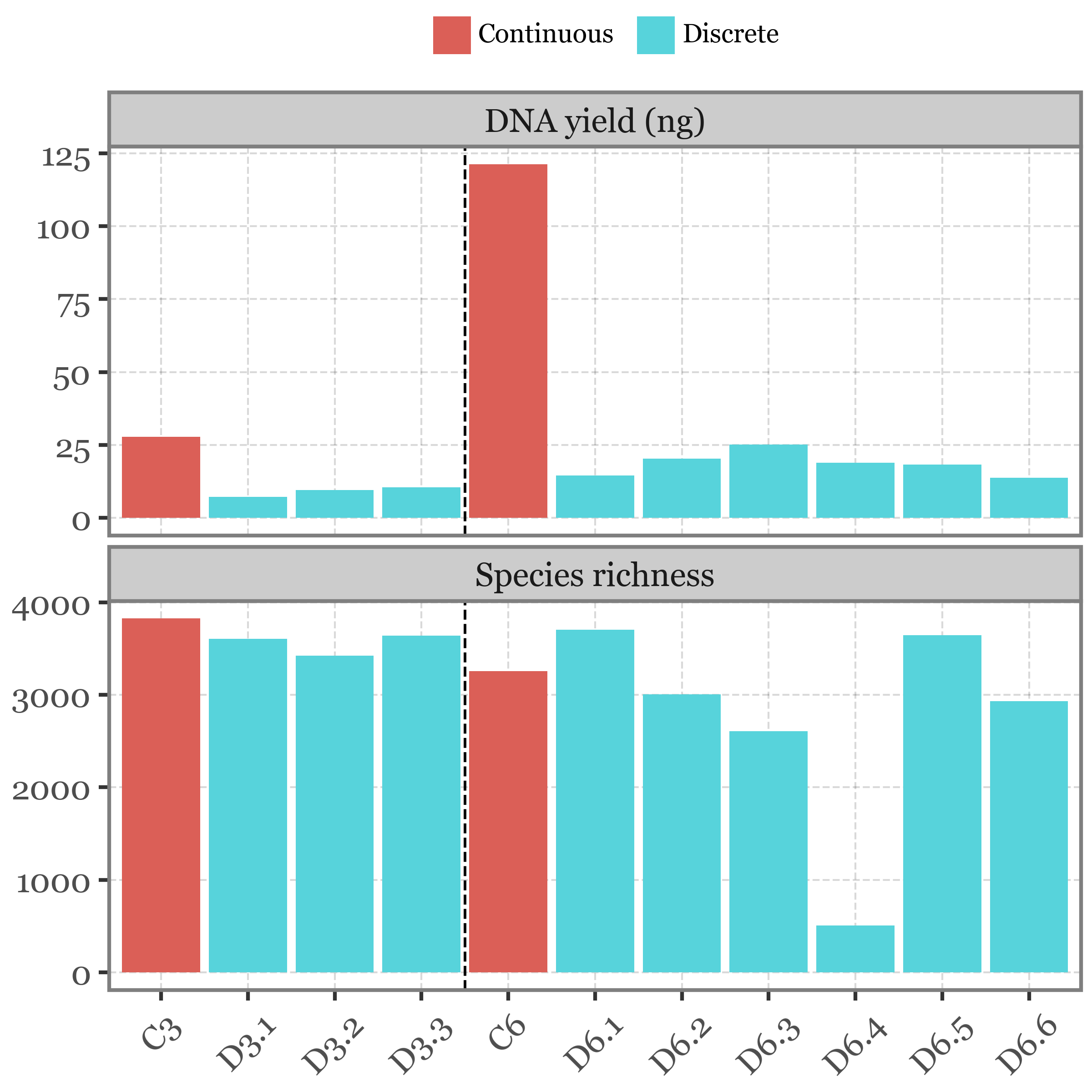
The continuous sampling method yields more DNA, which is expected given the longer sampling durations. However, this higher DNA yield does not correspond to increased species richness. On the contrary, discrete sampling, which yields lower DNA amounts, shows relatively high species richness.
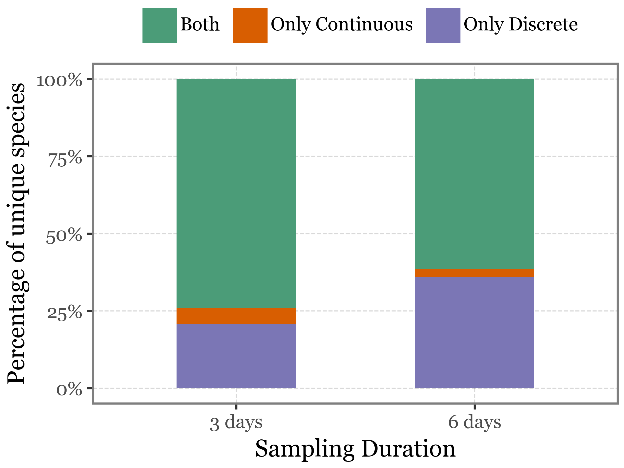
When we look beyond species richness to examine the specific species present in each sampling method, we see that, while most species are common to both approaches, about 25% of species are unique to discrete sampling, compared to only around 3% unique to continuous sampling suggesting that discrete sampling may capture a broader diversity of species.
Show Code
table_3 = (species_long
 .merge(exp_1_meta)
 .query('sampling_days.notna()')
 .query('reads > 0')
 .query('sampling_days == "3"')
 .groupby(['name', 'mode', 'sampling_days'])
 ['reads']
 .sum()
 .reset_index()
 .pivot(index='name', columns=['mode'], values='reads')
 .fillna(0)
 .loc[lambda x: x.sum(axis=1) > 0]
 .applymap(lambda x: x > 0)
 .assign(presence=lambda dd:
         np.where(dd['Continuous'] == dd['Discrete'], 'Both',
         np.where(dd['Continuous'], 'Only Continuous', 'Only Discrete'))
         )
 .dropna()
 .groupby(['presence'])
 .size()
 .reset_index()
 .rename(columns={0:'richness'})
 .assign(freq=lambda dd: dd['richness'] / dd['richness'].sum())
 .assign(days="3 days")
 )

table_6 = (species_long
 .merge(exp_1_meta)
 .query('sampling_days.notna()')
 .query('reads > 0')
 .query('sampling_days == "6"')
 .groupby(['name', 'mode', 'sampling_days'])
 ['reads']
 .sum()
 .reset_index()
 .pivot(index='name', columns=['mode'], values='reads')
 .fillna(0)
 .loc[lambda x: x.sum(axis=1) > 0]
 .applymap(lambda x: x > 0)
 .assign(presence=lambda dd:
         np.where(dd['Continuous'] == dd['Discrete'], 'Both',
         np.where(dd['Continuous'], 'Only Continuous', 'Only Discrete'))
         )
 .dropna()
 .groupby(['presence'])
 .size()
 .reset_index()
 .rename(columns={0:'richness'})
 .assign(freq=lambda dd: dd['richness'] / dd['richness'].sum())
 .assign(days="6 days")
 )


(pd.concat([table_3, table_6])
 .pipe(lambda dd: p9.ggplot(dd)
       + p9.aes('days', 'freq')
       + p9.geom_col(p9.aes(fill='presence'), width=.5)
       + p9.scale_y_continuous(labels=percent_format())
       + p9.scale_fill_manual(['#4B9C78', '#D85E01', '#7B76B5'

       ])
       + p9.labs(x='Sampling Duration', y='Percentage of unique species', fill='')
       + p9.theme(figure_size=(4, 3),
                  legend_position='top'
                  )


 )
       )
If we represent the same information in a Sankey diagram:
Show Code
Image('../output/sankey_3d_vs_6d.png')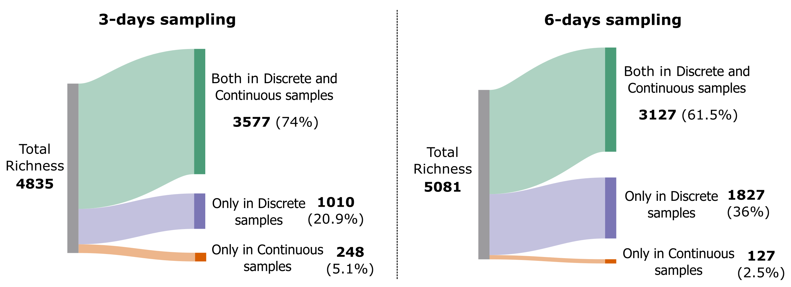
Experiment 2: PM10 vs PM2.5 heads
If we take a look now at the 3 daily samples taken with a PM10 head and the 3 daily samples taken with a PM2.5 head, focusing on the distribution of identified species in these samples:
Show Code
(species_long
.merge(metadata_df[['Sampling', 'Sample ID', 'sample_id']])
.rename(columns={'Sample ID': 'sample_code'})
.loc[lambda dd: dd.sample_code.str.contains('PM')]
.loc[lambda dd: dd.sample_code.str.endswith('-B')]
.loc[lambda dd: dd.sample_code.str.contains('.1.', regex=False)]
.assign(header=lambda dd: np.where(dd.sample_code.str.contains("2.5", regex=False),
                                   'PM2.5', 'PM10'
                                   ))
.query('reads > 0')
.pivot_table(index=['name'], columns='header', values='reads', aggfunc='sum')
.assign(presence=lambda dd: np.where(dd['PM10'].isna(), 'PM2.5',
                            np.where(dd['PM2.5'].isna(), 'PM10', 'Both')))
.presence.value_counts()
)
presence
Both 3634
PM10 841
PM2.5 740
Name: count, dtype: int64We see that in this case, from a total of 5215 species, 3634 appear in both types of samples, 841 are unique to PM10 samples and 740 are unique to PM2.5 samples.
I am going to now generate a table listing the species unique to each sample type and the count of unique samples where they appear. The formatted tables can be accessed here.
Show Code
uniquely_unique = (species_long
.merge(metadata_df[['Sampling', 'Sample ID', 'sample_id']])
.rename(columns={'Sample ID': 'sample_code'})
.query('name not in @contamination_list')
.loc[lambda dd: dd.sample_code.str.contains('PM')]
.loc[lambda dd: dd.sample_code.str.endswith('-B')]
.loc[lambda dd: dd.sample_code.str.contains('.1.', regex=False)]
.assign(header=lambda dd: np.where(dd.sample_code.str.contains("2.5", regex=False),
'PM2.5', 'PM10'
))
.query('reads > 0')
.groupby(['name', 'header'])
.size()
.rename('n_present')
.reset_index()
.pivot(index='name', columns='header', values='n_present')
.fillna(0)
.astype(int)
.query('`PM2.5`==0 or `PM10`==0')
.query('`PM2.5`>=1 or `PM10`>=1')
.index
.values
)
unique_pm_reads = (species_long
.merge(metadata_df[['Sampling', 'Sample ID', 'sample_id']])
.rename(columns={'Sample ID': 'sample_code'})
.query('name not in @contamination_list')
.loc[lambda dd: dd.sample_code.str.contains('PM')]
.loc[lambda dd: dd.sample_code.str.endswith('-B')]
.loc[lambda dd: dd.sample_code.str.contains('.1.', regex=False)]
.assign(header=lambda dd: np.where(dd.sample_code.str.contains("2.5", regex=False),
'PM2.5', 'PM10'
))
.query('reads > 0')
.query('name in @uniquely_unique')
.groupby(['name', 'header'])
.agg({'reads': sum, 'sample_code': 'nunique'})
.reset_index()
)
(unique_pm_reads
.pivot(index='name', columns='header')
.fillna(0)
.astype(int)
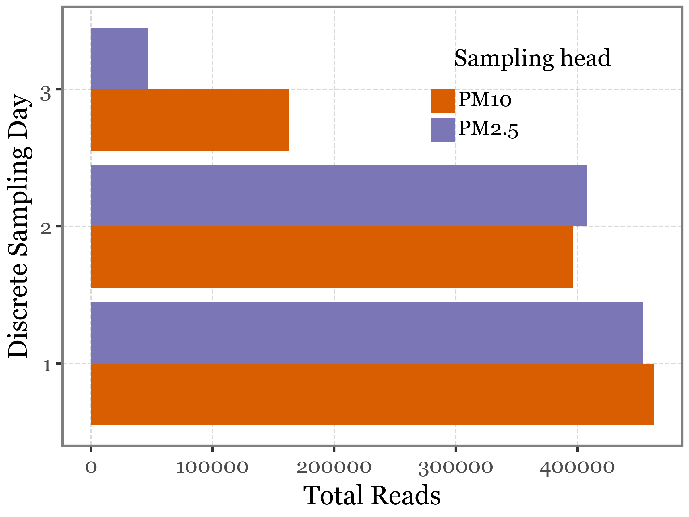
).to_csv('../output/table_unique_species_pm.csv')Upon reviewing the total number of reads assigned per sample day and head type, we observe that the number of reads detected on Days 1 and 2 is very similar for both heads. However, on the third day, the PM2.5 head shows a significantly lower number of reads compared to the PM10 head. This is an intriguing observation, as we would expect PM10 to include the PM2.5 fraction, suggesting that PM10 should have a higher mass. While this assumption holds true in terms of DNA yield, it is not reflected in two out of the three experiments.
Show Code
(species_long
.merge(metadata_df[['Sampling', 'Sample ID', 'sample_id']])
.rename(columns={'Sample ID': 'sample_code'})
.query('name not in @contamination_list')
.loc[lambda dd: dd.sample_code.str.contains('PM')]
.loc[lambda dd: dd.sample_code.str.endswith('-B')]
.loc[lambda dd: dd.sample_code.str.contains('.1.', regex=False)]
.assign(header=lambda dd: np.where(dd.sample_code.str.contains("2.5", regex=False),
                                   'PM2.5', 'PM10'
                                   ))
.query('reads > 0')
.groupby(['header', 'sample_code'])
.reads.sum()
.reset_index()
.assign(sample_code=lambda dd: dd.sample_code.str.split('-').str[0])
.assign(day=lambda dd: dd.sample_code.str.split('.').str[-1])
.pipe(lambda dd: p9.ggplot(dd)
      + p9.aes('day', 'reads', fill='header')
      + p9.geom_col(position='dodge')
      + p9.coord_flip()
      + p9.scale_fill_manual(['#D85E01', '#7B76B5'])
      + p9.labs(x='Discrete Sampling Day', y='Total Reads', fill='Sampling head')
      + p9.theme(
          figure_size=(4, 3),
          legend_position=(.8, .85),
          legend_key_size=10,
          legend_title=p9.element_text(x=80, y=50, size=10)
          )
      )
)
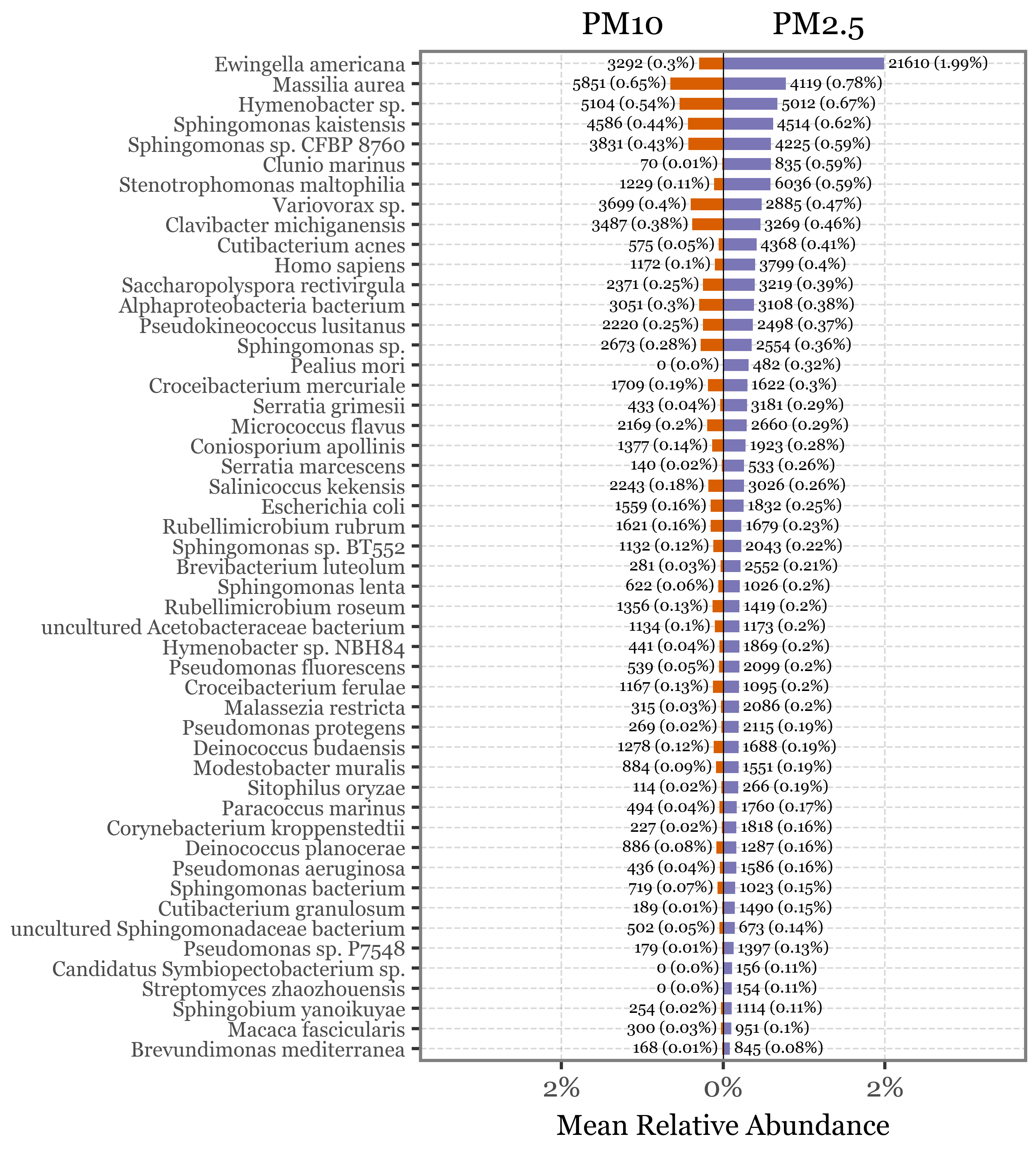
By focusing on species that are unique to each head type and present with higher relative abundance in one of the types, we can identify the top 50 most differentially abundant species. Our analysis reveals that the majority of the taxa more prevalent in the PM2.5 fraction compared to PM10 are bacterial species.
Show Code
species_by_header = (species_long
.merge(metadata_df[['Sampling', 'Sample ID', 'sample_id']])
.rename(columns={'Sample ID': 'sample_code'})
.query('name not in @contamination_list')
.loc[lambda dd: dd.sample_code.str.contains('PM')]
.loc[lambda dd: dd.sample_code.str.endswith('-B')]
.loc[lambda dd: dd.sample_code.str.contains('.1.', regex=False)]
.assign(header=lambda dd: np.where(dd.sample_code.str.contains("2.5", regex=False),
                                   'PM2.5', 'PM10'
                                   ))
.groupby(['header', 'sample_code'], as_index=False)
.apply(lambda dd: dd.assign(rel_abundance=lambda x: x['reads'] / x['reads'].sum()))
.reset_index(drop=True)
.groupby(['name', 'header'])
.agg({'rel_abundance': lambda x: x.sum() / 3, 'reads': 'sum'})
.loc[lambda x: x.reads > 0]
.reset_index()
.pivot(index='name', columns='header', values=['rel_abundance', 'reads'])
.fillna(0)
.assign(diff=lambda dd: (dd[('rel_abundance',  'PM2.5')] - dd[('rel_abundance',  'PM10')]))
.assign(direction=lambda dd: np.where(dd['diff'] > 0, 'PM2.5 > PM10', 'PM2.5 < PM10'))
.assign(abs_diff=lambda dd: dd['diff'].abs())
.sort_values('diff', ascending=False)
.head(50)
.assign(reads_label=lambda dd:
        dd['reads', 'PM10'].astype(int).astype(str) + ':' +
        dd['reads', 'PM2.5'].astype(int).astype(str))
.reset_index()
.assign(direction=lambda dd:
        pd.Categorical(dd.direction, categories=['PM2.5 > PM10', 'PM2.5 < PM10'],
                       ordered=True)
)
 .replace({"Candidatus Symbiopectobacterium sp. 'North America'":
           "Candidatus Symbiopectobacterium sp."})
)

sorted_species_rel = species_by_header.sort_values(('rel_abundance', 'PM2.5'))['name']
sorted_species_reads = species_by_header.sort_values(('reads', 'PM10'))['name']

species_by_header.columns = ['_'.join(col).strip() for col in species_by_header.columns.values]
(species_by_header
 .assign(rel_abundance_PM10=lambda dd: dd['rel_abundance_PM10'] * - 1)
 .assign(label_pm25=lambda dd: dd['reads_PM2.5'].astype(int).astype(str) +  ' ('
         + (dd['rel_abundance_PM2.5'] * 100).round(2).astype(str) + '%)')
 .assign(label_pm10=lambda dd: dd['reads_PM10'].astype(int).astype(str) +  ' ('
         + (dd['rel_abundance_PM10'].abs() * 100).round(2).astype(str) + '%)')
.assign(name=lambda dd: pd.Categorical(dd.name_, categories=sorted_species_rel, ordered=True))
.pipe(lambda dd: p9.ggplot(dd)
      + p9.aes('name')
      + p9.coord_flip()
      + p9.geom_col(p9.aes(y='rel_abundance_PM2.5'), fill='#7B76B5', width=.6)
      + p9.geom_col(p9.aes(y='rel_abundance_PM10'), fill='#D85E01', width=.6)
      + p9.geom_text(p9.aes(label='label_pm10', y='rel_abundance_PM10'),
                      size=5, ha='right', nudge_y=-.0005)
      + p9.geom_text(p9.aes(label='label_pm25', y='rel_abundance_PM2.5'),
                      size=5, ha='left', nudge_y=.0005)
      + p9.scale_y_continuous(
          labels=["2%", "0%", "2%"],
          limits=[-.034, .034])
      + p9.annotate('hline', yintercept=0, linetype='solid', size=.2)
      + p9.labs(x='', y='Mean Relative Abundance', title=f'PM10              PM2.5')
      + p9.theme(figure_size=(4.5, 5),
                 axis_text_y=p9.element_text(size=6.5),
                 axis_title_x=p9.element_text(size=9),
                 plot_title=p9.element_text(size=10, ha='center'),
                 )
      )
)
If we instead focus on the species that appear in at least 2 samples of one head type and none of the other, the top 30 for each head type are:
Show Code
f = (unique_pm_reads
     .query('sample_code >= 2')
 .groupby('header')
 .apply(lambda dd: dd
        .sort_values('reads', ascending=False)
        .reset_index(drop=True)
        .assign(rank=lambda x: x.index + 1)
        )
 .reset_index(drop=True)
 .query('rank <= 30')
 .replace({'PM10': 'Present only in PM10', 'PM2.5': 'Present only in PM2.5'})
 .pipe(lambda dd: p9.ggplot(dd)
       + p9.aes('reorder(name, reads)', 'reads')
       + p9.geom_col(p9.aes(fill='header'))
       + p9.facet_wrap('header', scales='free_y', ncol=1)
       + p9.coord_flip()
       + p9.labs(x='', y='')
       + p9.scale_fill_manual(['#D85E01', '#7B76B5'])
       + p9.guides(fill=False)
       + p9.theme(figure_size=(5, 7))

       )
)

f.save('../output/unique_pm_species.svg', dpi=300)
f.draw()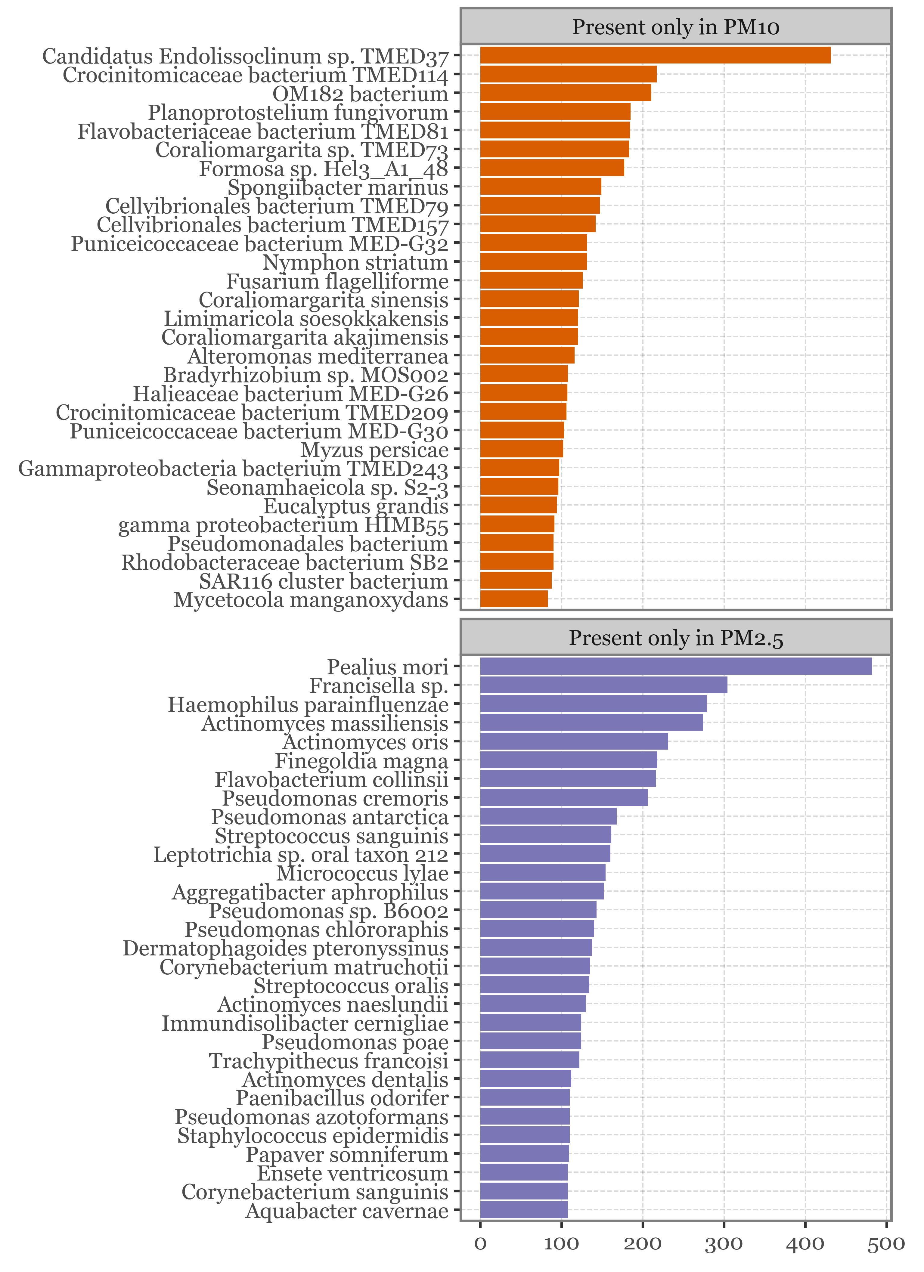
If we go ahead and test whether the richness of species is different between the two head types, we can do a non-parametric paired test (Wilcoxon signed-rank test) to compare the richness of species between the two head types:
24 * 7168Show Code
pm_richness = (species_long
.merge(metadata_df[['Sampling', 'Sample ID', 'sample_id']])
.rename(columns={'Sample ID': 'sample_code'})
.query('name not in @contamination_list')
.loc[lambda dd: dd.sample_code.str.contains('PM')]
.loc[lambda dd: dd.sample_code.str.endswith('-B')]
# .loc[lambda dd: dd.sample_code.str.contains('.1.', regex=False)]
.assign(header=lambda dd: np.where(dd.sample_code.str.contains("2.5", regex=False),
                                   'PM2.5', 'PM10'
                                   ))
.query('reads > 0')
.groupby(['header', 'sample_code'])
['name']
.nunique()
.reset_index()
.assign(day=['1 day (1)', '1 day (2)', '1 day (3)', '3 days', '6 days'] * 2)
.pivot(index='day', columns='header', values='name')
.assign(diff=lambda dd: (dd['PM2.5'] - dd['PM10']))
)

pm_richness| header | PM10 | PM2.5 | diff |
|---|---|---|---|
| day | |||
| 1 day (1) | 3682 | 3626 | -56 |
| 1 day (2) | 3019 | 3232 | 213 |
| 1 day (3) | 1599 | 642 | -957 |
| 3 days | 3725 | 3650 | -75 |
| 6 days | 1016 | 503 | -513 |
The results of the test show a non-significant difference in the richness of species between the two head types (p-value = 0.75).
(species_long
.merge(metadata_df[['Sampling', 'Sample ID', 'sample_id']])
.rename(columns={'Sample ID': 'sample_code'})
.loc[lambda dd: dd.sample_code.str.contains('PM')]
.loc[lambda dd: dd.sample_code.str.endswith('-B')]
.assign(header=lambda dd: np.where(dd.sample_code.str.contains("2.5", regex=False),
'PM2.5', 'PM10'
))
[['sample_id', 'sample_code', 'header']]
.drop_duplicates()
.merge(dna_yields)
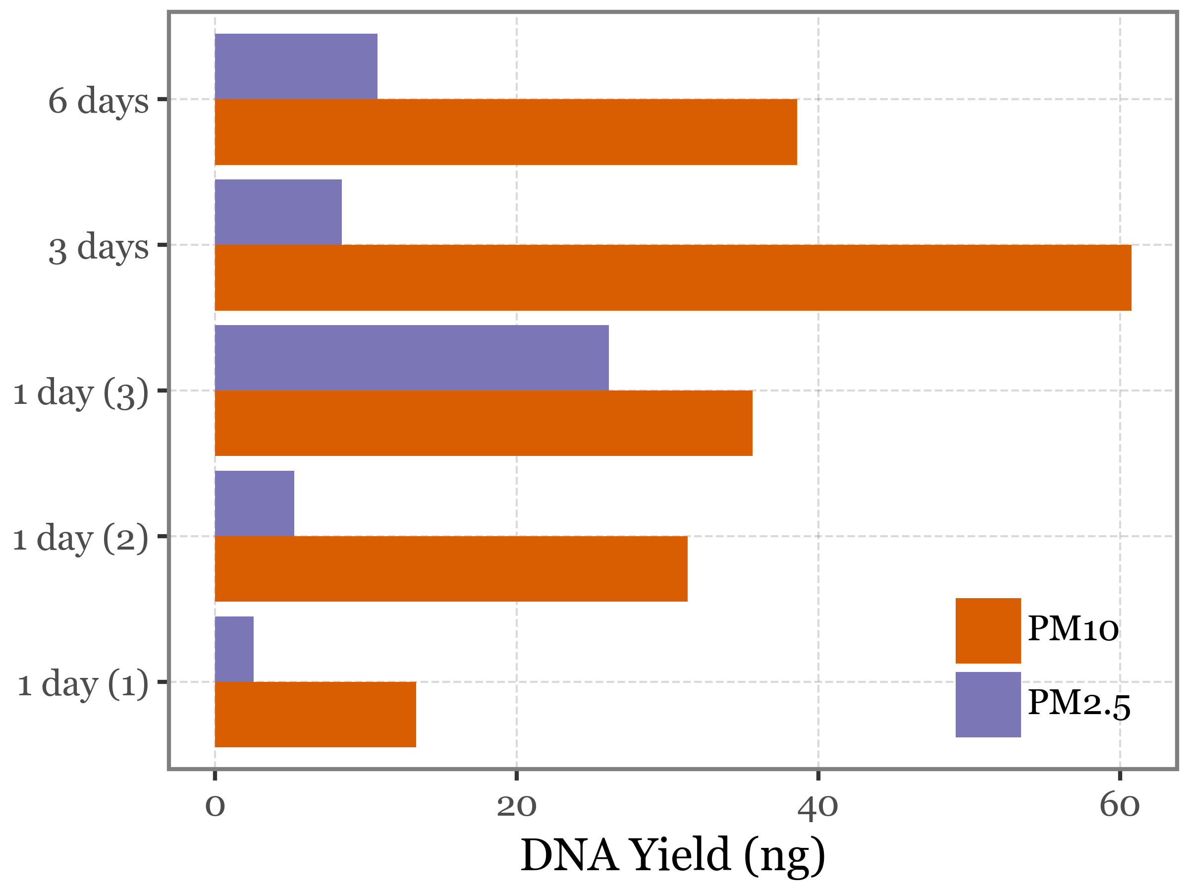
.assign(sample_comp=['3 days', '3 days', '6 days', '6 days', '1 day (1)'
, '1 day (1)', '1 day (2)', '1 day (2)', '1 day (3)', '1 day (3)'])
)| sample_id | sample_code | header | dna_yield | sample_comp | |
|---|---|---|---|---|---|
| 0 | HVSP22 | PM10.3-B | PM10 | 60.746667 | 3 days |
| 1 | HVSP23 | PM2.5.3-B | PM2.5 | 8.426333 | 3 days |
| 2 | HVSP49 | PM10.6-B | PM10 | 38.590000 | 6 days |
| 3 | HVSP50 | PM2.5.6-B | PM2.5 | 10.795000 | 6 days |
| 4 | HVSP51 | PM10.1.1-B | PM10 | 13.345000 | 1 day (1) |
| 5 | HVSP52 | PM2.5.1.1-B | PM2.5 | 2.567000 | 1 day (1) |
| 6 | HVSP53 | PM10.1.2-B | PM10 | 31.336667 | 1 day (2) |
| 7 | HVSP54 | PM2.5.1.2-B | PM2.5 | 5.264333 | 1 day (2) |
| 8 | HVSP55 | PM10.1.3-B | PM10 | 35.643333 | 1 day (3) |
| 9 | HVSP56 | PM2.5.1.3-B | PM2.5 | 26.123333 | 1 day (3) |
(species_long
.merge(metadata_df[['Sampling', 'Sample ID', 'sample_id']])
.rename(columns={'Sample ID': 'sample_code'})
.loc[lambda dd: dd.sample_code.str.contains('PM')]
.loc[lambda dd: dd.sample_code.str.endswith('-B')]
.assign(header=lambda dd: np.where(dd.sample_code.str.contains("2.5", regex=False),
                                   'PM2.5', 'PM10'
                                   ))
[['sample_id', 'sample_code', 'header']]
.drop_duplicates()
.merge(dna_yields)
.assign(sample_comp=['3 days', '3 days', '6 days', '6 days', '1 day (1)'
                     , '1 day (1)', '1 day (2)', '1 day (2)', '1 day (3)', '1 day (3)'])
.pipe(lambda dd: p9.ggplot(dd)
      + p9.aes('sample_comp', 'dna_yield', fill='header')
      + p9.geom_col(position='dodge')
      + p9.coord_flip()
      + p9.scale_fill_manual(['#D85E01', '#7B76B5'])
      + p9.labs(x='', y='DNA Yield (ng)', fill='')
      + p9.theme(figure_size=(4, 3),
                 legend_position=(.95, .05),)
)

    #   )

)
from scipy.stats import shapiro, ttest_rel, wilcoxon, ttest_ind, mannwhitneyu

# Updated dataset
extended_data = pd.DataFrame({
    'sample_id': ['HVSP22', 'HVSP23', 'HVSP49', 'HVSP50', 'HVSP51',
                  'HVSP52', 'HVSP53', 'HVSP54', 'HVSP55', 'HVSP56'],
    'sample_code': ['PM10.3-B', 'PM2.5.3-B', 'PM10.6-B', 'PM2.5.6-B', 'PM10.1.1-B',
                    'PM2.5.1.1-B', 'PM10.1.2-B', 'PM2.5.1.2-B', 'PM10.1.3-B', 'PM2.5.1.3-B'],
    'header': ['PM10', 'PM2.5', 'PM10', 'PM2.5', 'PM10',
               'PM2.5', 'PM10', 'PM2.5', 'PM10', 'PM2.5'],
    'dna_yield': [60.75, 8.42, 38.59, 10.79, 13.34,
                  2.57, 31.33, 5.26, 35.64, 26.12],
})

# Extract PM10 and PM2.5 data
pm10_yields = extended_data[extended_data['header'] == 'PM10']['dna_yield'].values
pm25_yields = extended_data[extended_data['header'] == 'PM2.5']['dna_yield'].values

# Normality test on paired differences
differences_extended = pm10_yields - pm25_yields
shapiro_test_extended = shapiro(differences_extended)

# Paired t-test
paired_t_test_extended = ttest_rel(pm10_yields, pm25_yields)

# Wilcoxon signed-rank test
wilcoxon_test_extended = wilcoxon(pm10_yields, pm25_yields)

# Unpaired t-test (Welch’s test)
unpaired_t_test_extended = ttest_ind(pm10_yields, pm25_yields, equal_var=False)

# Mann-Whitney U test
mannwhitney_test_extended = mannwhitneyu(pm10_yields, pm25_yields, alternative='two-sided')

# Print results
print("Shapiro-Wilk Normality Test:", shapiro_test_extended)
print("Paired t-test:", paired_t_test_extended)
print("Wilcoxon signed-rank test:", wilcoxon_test_extended)
print("Unpaired t-test:", unpaired_t_test_extended)
print("Mann-Whitney U test:", mannwhitney_test_extended)
Shapiro-Wilk Normality Test: ShapiroResult(statistic=0.8854308128356934, pvalue=0.33464905619621277)
Paired t-test: TtestResult(statistic=3.269238066491219, pvalue=0.03081127353194371, df=4)
Wilcoxon signed-rank test: WilcoxonResult(statistic=0.0, pvalue=0.0625)
Unpaired t-test: Ttest_indResult(statistic=2.9276970127016364, pvalue=0.02556940516470238)
Mann-Whitney U test: MannwhitneyuResult(statistic=24.0, pvalue=0.015873015873015872)(species_long
.merge(metadata_df[['Sampling', 'Sample ID', 'sample_id']])
.rename(columns={'Sample ID': 'sample_code'})
.loc[lambda dd: dd.sample_code.str.contains('PM')]
.loc[lambda dd: dd.sample_code.str.endswith('-B')]
.loc[lambda dd: dd.sample_code.str.contains('.1.', regex=False)]
.assign(header=lambda dd: np.where(dd.sample_code.str.contains("2.5", regex=False),
'PM2.5', 'PM10'
))
[['sample_id', 'sample_code', 'header']]
.drop_duplicates()
.merge(dna_yields)
.assign(sample_day=lambda dd: dd.sample_code.str[-5:-2])
)| sample_id | sample_code | header | dna_yield | sample_day | |
|---|---|---|---|---|---|
| 0 | HVSP51 | PM10.1.1-B | PM10 | 13.345000 | 1.1 |
| 1 | HVSP52 | PM2.5.1.1-B | PM2.5 | 2.567000 | 1.1 |
| 2 | HVSP53 | PM10.1.2-B | PM10 | 31.336667 | 1.2 |
| 3 | HVSP54 | PM2.5.1.2-B | PM2.5 | 5.264333 | 1.2 |
| 4 | HVSP55 | PM10.1.3-B | PM10 | 35.643333 | 1.3 |
| 5 | HVSP56 | PM2.5.1.3-B | PM2.5 | 26.123333 | 1.3 |
(metadata_df
 [['Sampling', 'Sample ID', 'sample_id']]
 .assign(header=lambda dd: np.where(dd.sample_id.str.contains("2.5", regex=False),'PM2.5', 'PM10')
 )
)| Sampling | Sample ID | sample_id | header |
|---|
stats.wilcoxon(pm_richness['diff'])WilcoxonResult(statistic=2.0, pvalue=0.75)Supp. Experiment: Bags vs Vial blanks
We are going to compare the richness of the blanks using vials and bags to see if there is a significant difference between the two types of blanks:
bag_vial_blanks = ['B6-B', 'B6-V', 'B3-B', 'BPM-B', 'B3-V', 'BPM-V', 'BQZ-B', 'BQZ-V']blanks_table = pd.read_csv('../data/ABS_hvs_blank2-sp.csv')
blanks_table.columns = [col.split('.')[0] for col in blanks_table.columns]
blanks_table.rename(columns={'#Datasets': 'name'}, inplace=True)Show Code
blanks_richness =(blanks_table
 .melt('name', var_name='sample_id', value_name='reads')
 .merge(metadata_df[['Sample ID', 'sample_id']])
 .query('`Sample ID` in @bag_vial_blanks')
 .assign(kind=lambda dd: dd['Sample ID'].str.split('-').str[1]
         .replace({'B': 'Bag', 'V': 'Vial'}))
 .assign(sample_name=lambda dd: dd['Sample ID'].str.split('-').str[0])
 .query('reads > 0')
 .groupby(['sample_name', 'kind'])
 .agg({'name': 'nunique'})
 .reset_index()
)

(blanks_richness
 .pipe(lambda dd: p9.ggplot(dd)
        + p9.aes('sample_name', 'name', fill='kind')
        + p9.geom_col(position='dodge', width=.7)
        + p9.coord_flip()
        + p9.labs(x='', y='Species Richness', fill='')
        + p9.scale_fill_manual(['#D85E01', '#7B76B5'])
        + p9.theme(figure_size=(4, 3),
                   legend_position='top',
                   legend_key_size=11,
                   )
       )
)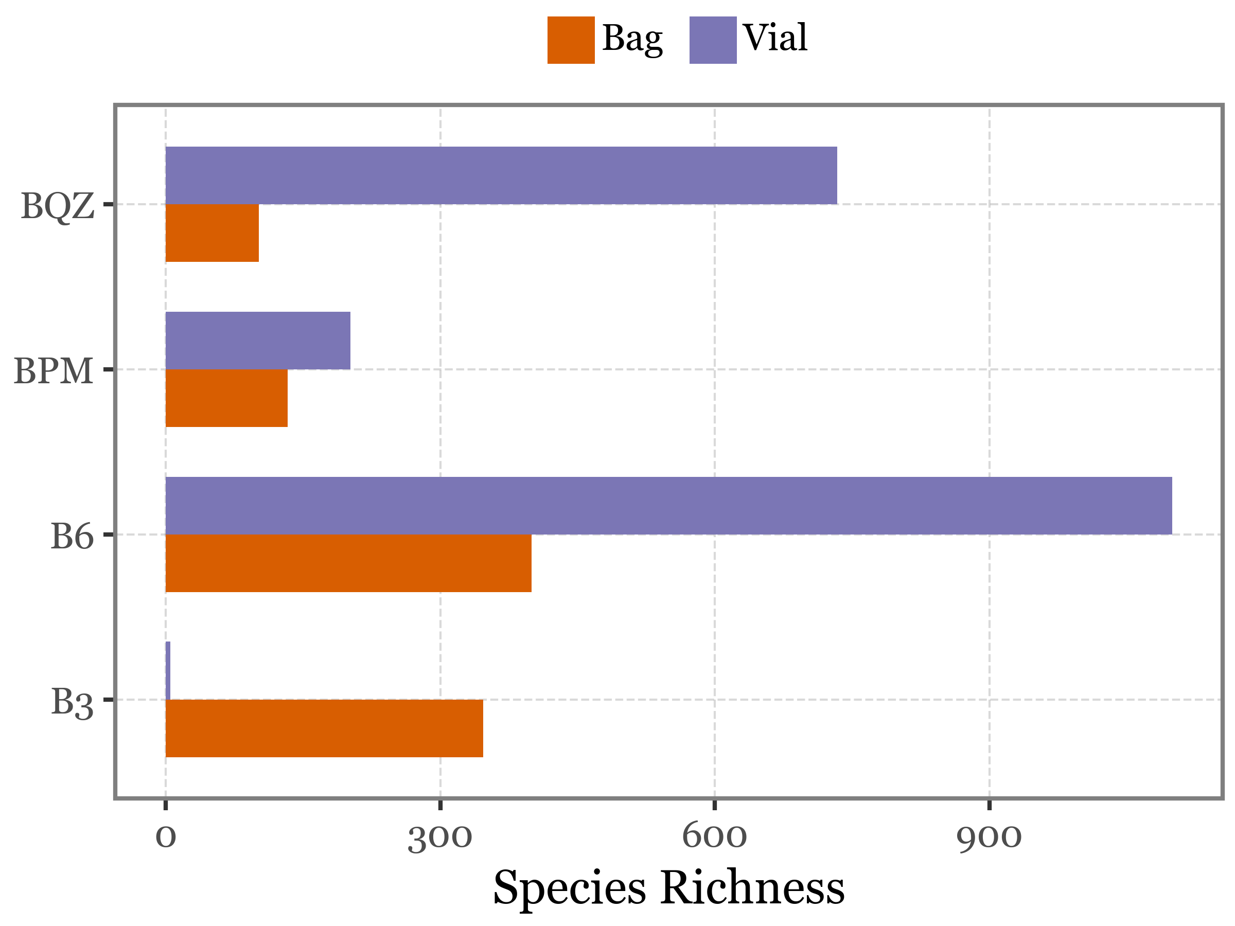
There is no significant difference when testing with a Wilcoxon signed-rank test (p-value = 0.375):
blanks_richness_diffs = (blanks_richness
.pivot(index='sample_name', columns='kind', values='name')
.eval('diff = Vial - Bag')
)
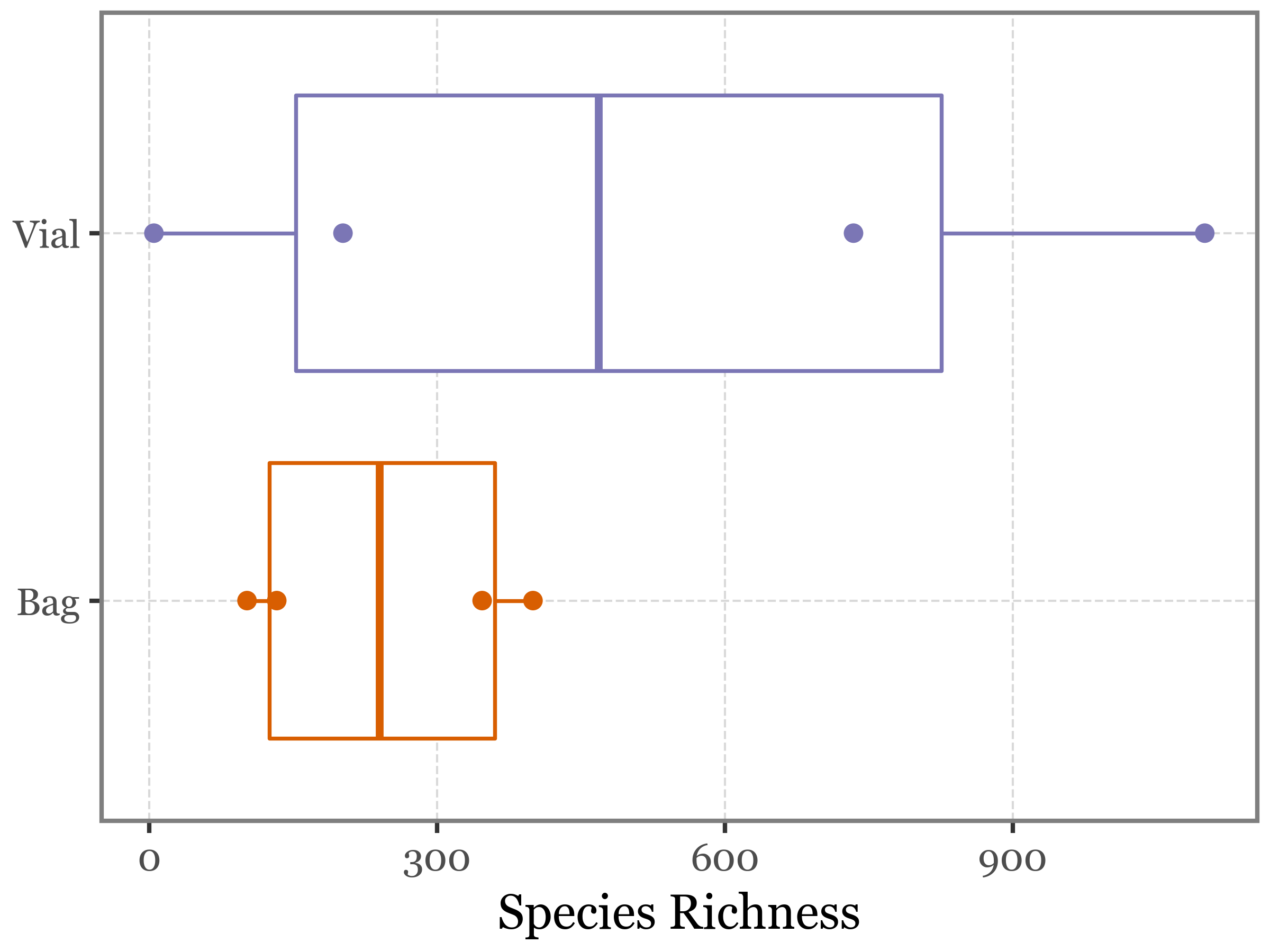
blanks_richness_diffs.pipe(lambda dd: stats.wilcoxon(dd['diff']))WilcoxonResult(statistic=2.0, pvalue=0.375)We can represent this comparison also with a boxplot:
Show Code
blanks_richness.pipe(
    lambda dd: p9.ggplot(dd)
    + p9.aes(x='kind', y='name', color='kind')
    + p9.geom_boxplot()
    + p9.geom_point()
    + p9.coord_flip()
    + p9.scale_color_manual(['#D85E01', '#7B76B5'])
    + p9.theme(figure_size=(4, 3))
    + p9.guides(color=False)
    + p9.labs(x='', y='Species Richness')
)
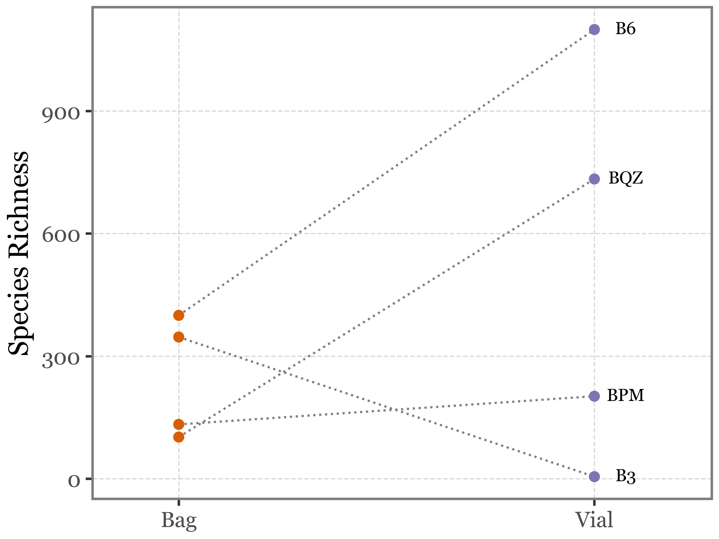
Or with a lineplot showing the paired differences:
Show Code
blanks_richness.pipe(
    lambda dd: p9.ggplot(dd)
    + p9.aes(x='kind', y='name', color='kind')
    + p9.geom_line(p9.aes(group='sample_name', y='name'), color='gray', linetype='dotted')
    + p9.geom_point()
    + p9.scale_color_manual(['#D85E01', '#7B76B5'])
    + p9.geom_text(p9.aes(label='sample_name'), nudge_x=.075, size=7,
                    data=dd.query('kind == "Vial"'), color='black')
    + p9.theme(figure_size=(4, 3))
    + p9.guides(color=False)
    + p9.scale_x_discrete(expand=(.1, .1))
    + p9.labs(x='', y='Species Richness')
)
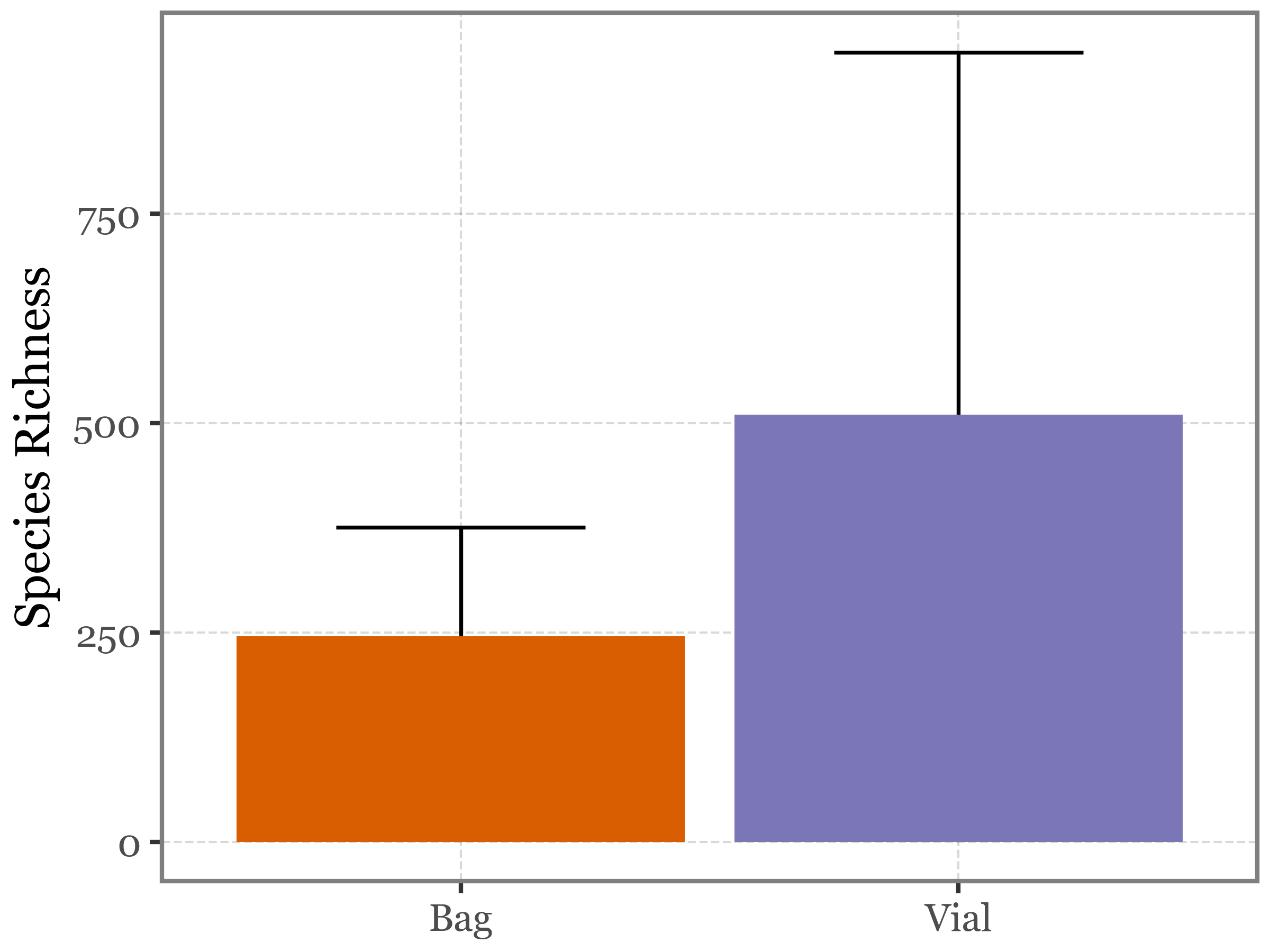
A classical barplot would look like this (but it’s not very informative since it obscures the paired nature of the data):
Show Code
(blanks_richness.pipe(
    lambda dd: p9.ggplot(dd)
    + p9.aes(x='kind', y='name', fill='kind')
    + p9.stat_summary(geom='errorbar',
                    fun_ymax=lambda x: np.mean(x) + np.std(x),
                    fun_ymin=lambda x: np.mean(x) - np.std(x),
                    width=.5)
    + p9.scale_fill_manual(['#D85E01', '#7B76B5'])
    + p9.guides(fill=False)
    + p9.stat_summary(geom='col', fun_y=np.mean)
    + p9.theme(figure_size=(4, 3))
    + p9.labs(x='', y='Species Richness')
)
)
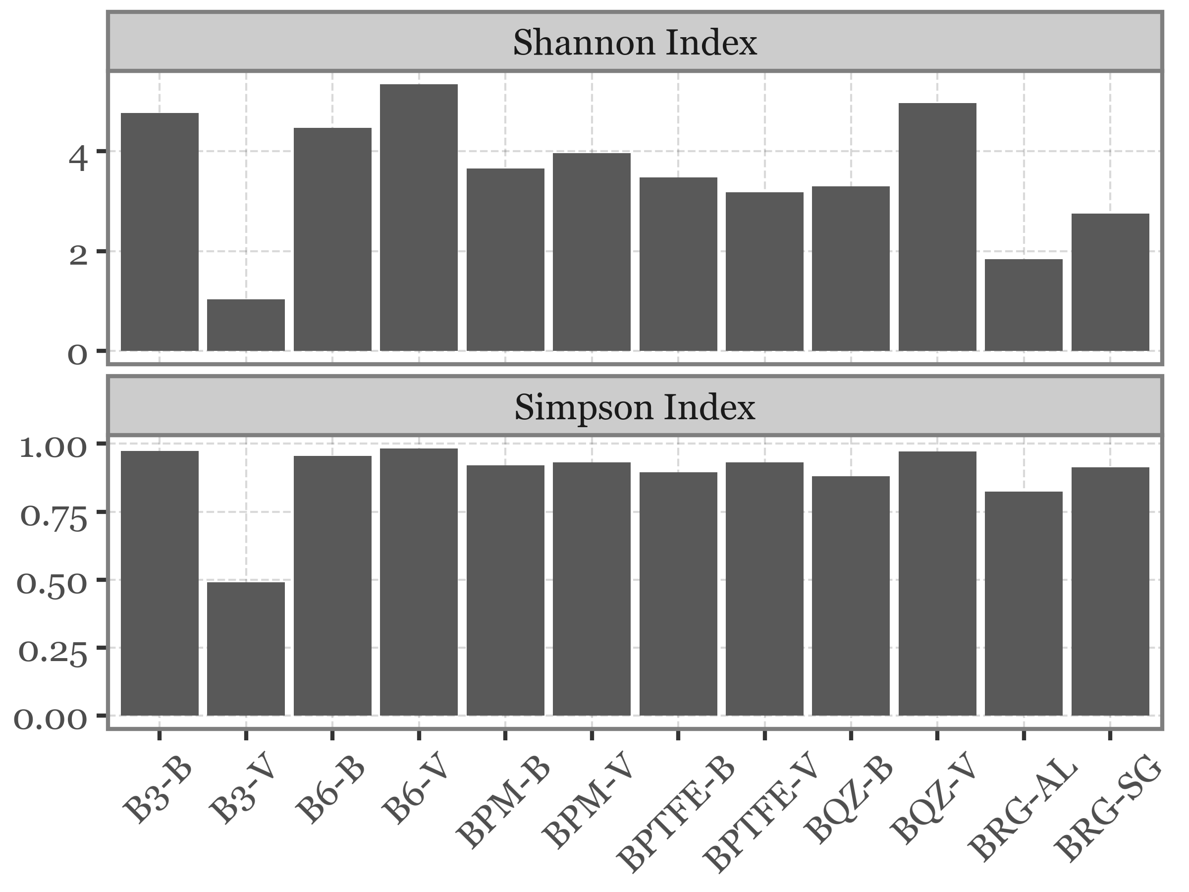
Shannon and Simpson diversity indexes
We are now going to compute the Shannon and Simpson diversity indexes for the blanks.
The Shannon diversity index H is given by the formula:
\[H = -\sum_{i=1}^{R} p_i \ln(p_i)\]
where:
- \(R\) is the total number of species,
- \(p_i\) is the proportion of individuals belonging to the \(i\)-th species, calculated as \(p_i = \frac{n_i}{N}\) ,
- \(n_i\) is the number of individuals in the i -th species,
- \(N\) is the total number of individuals across all species.
The Simpson diversity index D can then be defined as:
\[D = 1 - \sum_{i=1}^{R} p_i^2 = 1 - \frac{\sum_{i=1}^{R} n_i (n_i - 1)}{N (N - 1)} \]
We’ll define a function to calculate each of these indexes in numpy and then simply apply it to the columns of the dataframe with the species counts to get the diversity indexes for each sample:
from typing import List

def shannon_diversity(species_counts: List[int]) -> float:
    species_counts = np.array(species_counts)
    species_counts = species_counts[species_counts > 0]
    total_counts = np.sum(species_counts)
    proportions = species_counts / total_counts
    shannon_index = -np.sum(proportions * np.log(proportions))
    return shannon_index

def simpson_diversity(species_counts: List[int]) -> float:
    species_counts = np.array(species_counts)
    total_counts = np.sum(species_counts)
    proportions = species_counts / total_counts
    simpson_index = 1 - np.sum(proportions ** 2)
    return simpson_index
Show Code
blank_sample_names = metadata_df.loc[metadata_df['Sample ID'].str.startswith('B')]['Sample ID']

(blanks_table
 .melt('name', var_name='sample_id', value_name='counts')
 .merge(metadata_df[['Sample ID', 'sample_id']])
 .query('`Sample ID` in @blank_sample_names')
 .pivot(index='name', columns='Sample ID', values='counts')
 .fillna(0)
 .pipe(lambda dd: pd.concat([
        dd.apply(shannon_diversity, axis=0).rename('Shannon Index').reset_index()
        .merge(dd.apply(simpson_diversity, axis=0).rename('Simpson Index').reset_index())
    ])
 )
 .melt('Sample ID', var_name='index', value_name='value')
 .query('`Sample ID` != "BHVS-SG"')
 .pipe(lambda dd: p9.ggplot(dd)
       + p9.aes('Sample ID', 'value')
       + p9.geom_col()
       + p9.facet_wrap('~index', scales='free_y', ncol=1)
       + p9.labs(x='', y='')
       + p9.theme(figure_size=(4, 3), axis_text_x=p9.element_text(angle=45))
 )
)